Prediction Error

... how to accurately measure it?

When assessing the quality of a model, it is essential to accurately measure its prediction error. Otherwise, a model may fit the training data very well, but will do a poor job of prediction for ‘new’ data - the phenomenon of overfitting.

The primary goal while building predictive models must be to make it accurately predictive of the desired target value for ‘new’ data. In practice, a measure of model error is reported that is based not on the error for ‘new’ data, instead on the error for data used to train the model. This yields misleading results and the error the model exhibits on ‘new’ data is higher than that on the training data.

As an example, if we sample 100 people and create a regression model to predict an individual's happiness based on their wealth, we can record the squared error for how well the model does on this training set. Then if we sampled a different 100 people from the population and applied our model to this ‘new’ set, the squared error will almost always be higher.

Prediction Error = Training Error + Training Optimism

Higher the optimism, worse is the training error approximation to the prediction error. It turns out that the optimism is a function of model complexity.

Prediction Error = Training Error + f(Model Complexity)

As model complexity increases (e.g. adding parameters in linear regression) the model will do a better job fitting the training data, thereby reducing training error. This is a fundamental property of statistical models. Actually, no matter how unrelated the additional factors are to a model, adding them will decrease the training error. At the same time, as we increase model complexity we can see a change in the prediction error. Even adding relevant factors to the model can increase the prediction error, if the signal-to-noise ratio of those is weak.

In the happiness and wealth regression model, if we start with the simplest and then increase complexity by adding nonlinear (polynomial) terms, what we get is something like the following:

Happiness = a + b(Wealth) + ϵ

Happiness = a + b(Wealth) + c(Wealth^2) + ϵ

& so on…

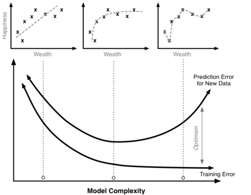
The linear model (minus polynomial terms) seems a little too simple for the data, but once we pass a certain point, the prediction error starts to rise. The additional complexity helps us fit our training data, but causes the model to do a worse job of predicting for ‘new’ data. This is a clear case of overfitting the train data. Preventing overfitting is key to building robust and accurate predictive models.

Methods for Accurate Measurement of Prediction Error

Here we discuss some techniques to accurately measure prediction error. In general, assumption-based (parametric) approaches are faster to apply, but come at a high cost. How much of the assumptions skews the results varies on a case by case basis. The error might be negligible in many cases, but fundamentally results derived from such techniques require a great deal of trust on the evaluator’s part.

On the other hand, the primary cost of cross-validation resampling approach is computational intensity. It however provides more confidence and security in the resulting conclusions.

Choosing a method is mainly based on whether we want to rely on assumptions to adjust for the optimism, or we want to use the data for estimating the optimism.

1. Adjusted R^2

It is based on parametric assumptions that may or may not be true in a specific application. Adjusted R² does not perfectly match up with (true) prediction error, it in general under-penalizes model complexity that is, it fails to decrease the error as much as is required with the addition of complexity in the model. This can lead to misleading conclusions. However, it is fast to compute and easy to interpret.

For details on R^2 and adjusted R^2, please read this article.

2. Information Theory

Information theoretic approaches assume a parametric model wherein, we can define the likelihood of a dataset and its parameters. If we adjust the parameters in order to maximize this likelihood we obtain the maximum likelihood estimate of the parameters for a given model and dataset. In other words, these approaches attempt to measure model error as how much information is lost between a candidate model and the true model. The true model (what was used to generate the data) is unknown, but given certain assumptions we can obtain an estimate of the difference between it and and our proposed models. More this difference is, higher the error and worse the candidate (tested) model.

Akaike's Information Criterion (AIC) is defined as a function of the likelihood of a model and the number of parameters (m) in that model.

AIC = −2ln(likelihood) + 2m

Then there is Bayesian Information Criterion (BIC) for sample size n.

BIC = −2ln(likelihood) + mln(n)

The first term in the equation can be thought of as the training error and the second term can be thought of as the penalty to adjust for the optimism. The goal is to minimize AIC. These measures/metrics hence require a model that can generate likelihoods, thereby needing a leap of faith that the specific equation used is theoretically suitable to the problem and associated data.

3. Holdout Set

By holding out a test dataset from the beginning, we can directly measure how well the model will predict for new data. This is a non-parametric approach and a gold standard to measure the prediction error.

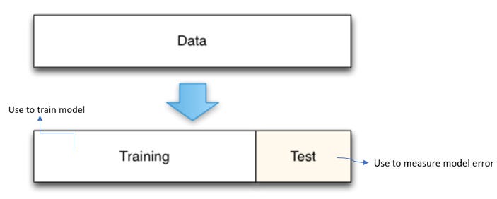
A common mistake is to create a holdout set, train a model, test it on the holdout set, and then adjust the model in an iterative process. If the holdout set is repeatedly used to test a model during development, the holdout set becomes contaminated. It has been used as part of the model selection process and no longer yields unbiased estimates of the (true) prediction error. Given enough data, this metric is highly accurate, it is furthermore conceptually simple and easy to implement. It has a potential conservative bias, it’s useful in practice nonetheless compared to overly optimistic predictions.

4. Cross-validation

The obvious issue in having a validation subset of data is that our estimate of the test error can be highly variable, depending on which particular observations are included in the training subset and which are included in the validation set. That is, how do we know what’s best way (or percent) to split the data?

Another issue with the approach is that it tends to overestimate the test error for models fit on our entire dataset. More training data usually means better accuracy, but the validation set approach reserves a decent-sized chunk of data for validation and testing.

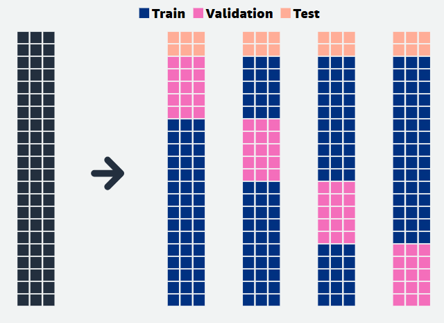
We should come up with a way to use more of our data for training while also simultaneously evaluating the performance across all the variance in our data. And that’s a resampling approach. Cross-validation (CV) works by splitting the data into n folds of equal size. Then the model building and error estimation process is repeated n times.

1. CV with hold-out set

5-fold CV

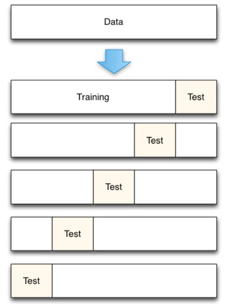
For a 5-fold CV, each time 4 of the groups are combined and used to train the model. The 5th group that was not used to construct the model is used to estimate the prediction error, ending up with 5 error estimates that are averaged to obtain a robust estimate of the prediction error.

Each data point is used both to train and test model, but never at the same time. When data is limited, CV is preferred to the holdout set method. CV also gives estimates of variability of the prediction error which is a useful feature.

Smaller the number of folds, more biased are the error estimates (conservative indicating higher error than there is, in reality). Hence, another factor to consider is computational time which increases with the number of folds and when it seems prudent to use a small number of folds. Choosing the fold size (or number of folds) may be a con of the CV approach, it nevertheless provides good error estimates with minimal assumptions.

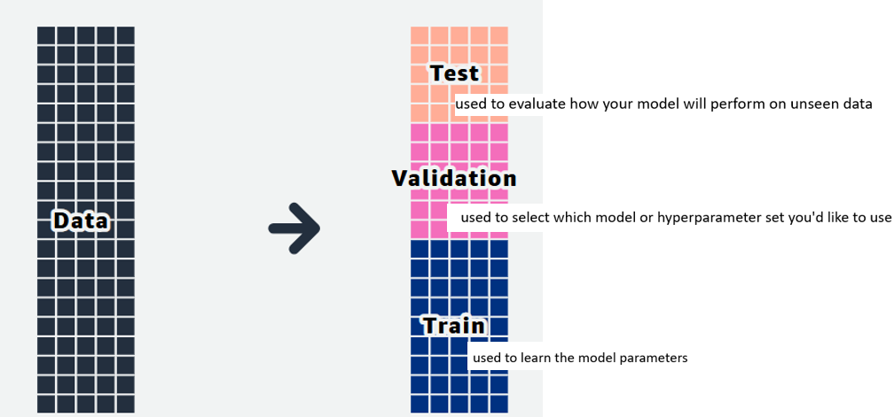
2. CV with validation set

   The training set (n-1 folds) will fit our model's parameters, and the validation set (1 fold) will be used for evaluation. This process will be repeated on our data n times, using a different fold for the validation set at each iteration. At the end of the procedure, we'll take the average of the validation sets' scores and use it as our model's estimated performance.

Note that the test data remains untouched as it’s the final hold-out set (used only once), but the distribution of training and validation sets differs at every fold.

The CV approach typically does not overestimate the test error as much as the validation set approach could for small training dataset sizes.

📌 Bias-variance tradeoff

How do different values of n affect the quality of evaluation estimates?

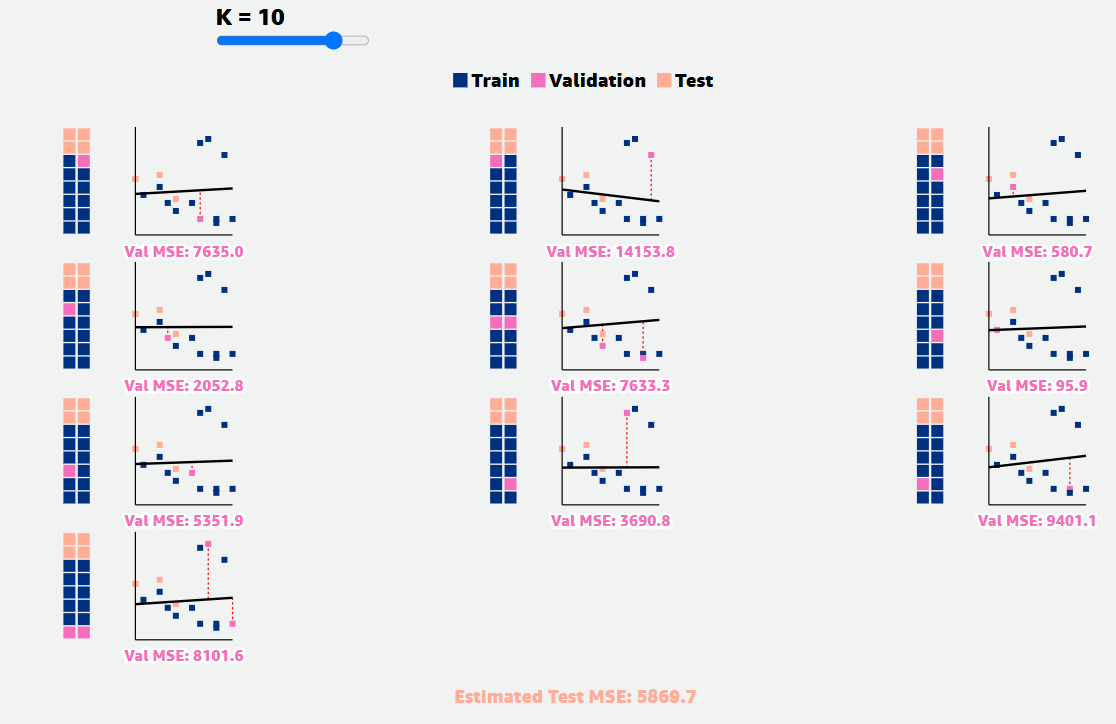
The lines of best fit and estimated test Mean Squared Error (MSE) vary more for lower values of n than for higher values of n. This is a consequence of the bias-variance tradeoff.

If understanding the variability of prediction error is important, resampling methods such as bootstrapping can be superior. Bagging (bootstrap aggregating) ensemble models (e.g. random forest) reduce variance.