


While preparing data to train some machine learning models, we transform a skewed variable (skewed distribution) into something very close to the Gaussian or normal distribution. Why is it justified?
Well, such a transformation helps justify the use of normal distributions in real-world scenarios when the underlying data distribution is unknown, or at the most their mean & variance can be estimated. The first four (excluding zero) moments of a distribution are mean, variance, skewness, and kurtosis in that order. The first moment is the center of mass of a (probability) distribution. Various distributions can satisfy the same moments but differ significantly in how they distribute outcomes, pretty much like the fact that two distributions with the same mean and variance can have different skewnesses.
The normal distribution maximizes entropy (randomness/uncertainty) with specified mean (μ) and variance (σ²) by optimally allocating probability mass (discrete random variable); allocation of probability density is done for a continuous random variable. For more on PMF and PDF, please visit the page.
A normal (symmetric) distribution has zero skewness. Normality ensures that the distribution function f(x) approaches zero as x moves further away from the mean, which reflects the decreasing likelihood of deviating far from the mean μ. The simplest normal distribution is the standard normal distribution which has zero mean and unity standard deviation (SD = σ).
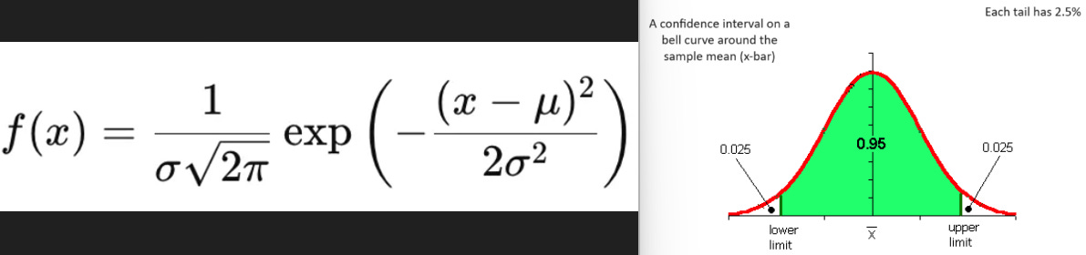
Let me dive in deeper. The numerator of the exponent in the function f(x) demonstrates the following:
Symmetry: The squared term is always positive and becomes zero when x is equal to μ. This means that the function reaches its maximum value when x = μ, ensuring the distribution is symmetric about its mean. This is crucial because it reflects the idea that deviations from the mean are equally likely in both directions. The quadratic form creates a parabolic curve when plotted which is essential for a bell shape of the distribution. The nature of a parabola is such that values close to the mean have higher probabilities and as you move away from the maximum, the probability density decreases exponentially. The smooth decrease in probability density is essential for modeling continuous data where extreme values are possible but become progressively less likely.
Penalization of extreme values: The quadratic term grows rapidly as x moves away from μ. This rapid growth means that values far from the mean (extreme values) are less likely than values close to the mean, which is a key characteristic of many natural phenomena.
The denominator (σ²) of the exponent in the function acts as a scaling factor. It influences the curve’s spread in the following way:
Small variance - means the data points are closely clustered around μ, resulting in a steeper (narrower, taller) curve. It causes the function f(x) to decrease faster as x deviates from the mean μ.
Large variance - means larger variability. It spreads the data points more broadly around the mean μ, resulting in a wider and flatter curve. It causes the function f(x) to decrease more slowly as x moves away from μ allowing for a higher dispersion of data points.
A normal distribution’s utility spans from hypothesis testing where it helps in constructing confidence interval (CI) to many others. A symmetric (bell-shaped) CI means that the point estimate lies in the centre of the CI. For example (see fig. 1), a 95% confidence level means that if you repeat an experiment/survey over and over again, 95% of the time your results will match the results obtained from a population.
A Gaussian curve also gives us the methodology Six Sigma - a fraction of the normal curve that lies within 6 SDs of the mean. This methodology originates from statistical quality control in manufacturing/business processes and is used to evaluate process capability. Six Sigma strategies seek to improve production and process quality by identifying causes of defects/errors, removing them and minimizing variability. Adopting the 6σ approach essentially implies the following:

A normal distribution underlies the statistical assumptions of 6σ. Zero marks the mean (horizontal axis in fig. 2 has units of SD). The greater the SD, the larger the spread of values. The upper and lower specification limits (USL, LSL) are at a distance of 6σ from the mean. Normal distribution means that values far away from the mean are extremely unlikely. Even if the mean were to move right or left by 1.5 SDs - also known as 1.5 sigma shift, there is still a safety cushion. The role of the sigma shift is mainly academic. The purpose of the 6σ methodology is to generate organizational performance improvement. It is up to the organization to determine, based on customer expectations, what the appropriate sigma level of a process is which serves as a comparative figure to determine whether a process is improving, deteriorating, stagnant or non-competitive with others in the same business.

One must note that the calculation of sigma level for process data is independent of the data being normally distributed. Practitioners using this approach spend a lot of time transforming data from non-normal to normal. However, sigma levels can be determined for non-normal data.
What kind of ML models need their input variables to be transformed to Gaussian distributions?
Parametric models have some assumptions in place, like the normality of residuals (errors which are the differences between predictions and actuals), the equation being linear in the coefficients of predictor variables. Independent variables if skewed usually undergo transformation (equation remaining linear in the parameters) while training linear models like regression, ANOVA test just so the conclusions drawn from them are more reliable.
Non-parametric models like kNN (decision tree-based algorithms etc.) do not need normality of input variables in the dataset. A variable transformation is usually not required while training non-linear models. Yet, predictions from such models often become reliable when the independent variables are normal or near-normal.
As such, variables with skewed distributions or different distributions altogether are transformed to our much-known Gaussian distributions which seem to stabilize the distribution’s second moment that is, the variance.