

Linear regression is a supervised learning algorithm, aims to explain the relationship between one (or more) independent variable (s) and a dependent variable (response/target). The coefficients (weights) on the independent variables are what the model learns during optimization. A linear regression model is trained by either ordinary least squares (OLS) fitting/optimization method or gradient descent.
A measure to assess the goodness of fit to data is called the coefficient of determination, as it determines how well the numeric predictions approximate the true data points. There’s an irreducible error term in the regression equation that collects all the unmodeled parts of the data.
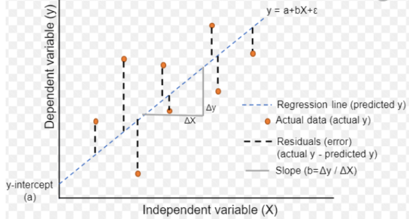
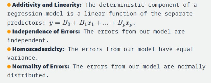
✅ Assumptions in linear regression
There’s more than one method to optimize as well as regularize the regression algorithm.
📌 Optimization methods
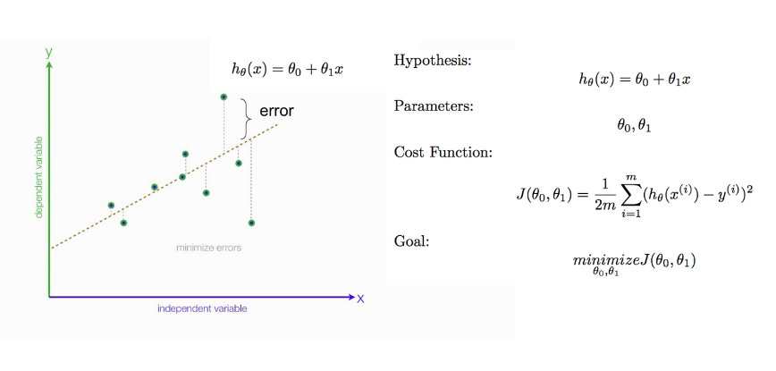
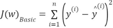
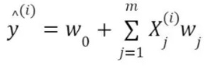
The OLS algorithm minimizes the sum of squared errors (SSE) wherein the cost or loss function is mean squared error (MSE = SSE/n) and optimization occurs in closed form. In fig.1 below, number of independent variables is m, the number of observations/rows in the dataset is n, and the y-intercept is also called the bias. The squaring of errors prevents negative and positive terms from canceling out in the sum and gives more weight to points further from the regression line, punishing outliers.
If the errors follow a normal distribution, OLS becomes MLE (maximum likelihood estimation) providing a probabilistic framework to draw inference from model estimates.
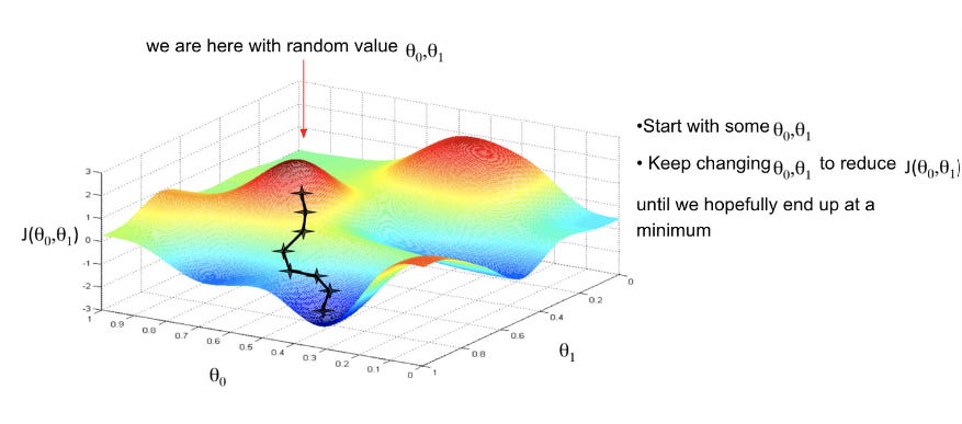
The gradient descent algorithm is an iterative process and minimizes the loss function by calculating the function derivative/slope and updating the weight/parameter after each iteration. This method therefore enables learning by making corrective updates to the estimates that move towards an optimal combination of parameters.
A demo of linear regression optimized with gradient descent is here. Post training a model, we might observe overfitting (the algorithm captures noise in the data), regularization of features helps reduce variance. Regularization prevents overfitting by not generating high coefficients for sparse predictor variables, also stabilizes the estimates especially when there's collinearity in data.
For an algorithm that involves non-convex optimizations (ones with local minima and maxima) adding (independent) variables could make it complex, harder to find the best set of model parameters and result in higher bias. However, for algorithms like linear regression with efficient and precise machinery, added variables will only always reduce bias.
📌 Regularization methods
Explicit regularization is where one explicitly adds a term to the (often ill-posed) optimization problem. These terms could be priors, or constraints. The regularization or penalty term imposes a cost on the optimization function to make the optimal solution unique. Explicit regularization of regression models almost always ensures optimal model complexity. Implicit regularization includes early stopping which is prevalent in stochastic gradient descent algorithm used for training/optimizing deep neural networks.
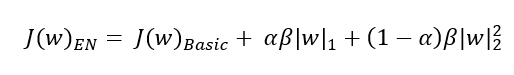
Regularized regression models, Lasso (L1) and Ridge (L2) are used for feature selection and reducing complexity of the model thereby enhancing model interpretability. There's a third type - ElasticNet that allows a balance of both L1 & L2 penalty terms, leading to better model performance in some cases.
A regression model is represented by a number of columns (m), a number of rows (n) in the dataset and regression coefficients or weights (w) on the independent variables. The loss function J in a vanilla (basic) linear model is a squared term. It is the square of the deviation of predicted value from actual value.
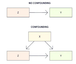
The terms ‘regressor’ (predictor or independent or explanatory variable) and ‘covariate’ may be used interchangeably, except that the latter must be used when there’s potential confounding. The following diagram explains confounding:
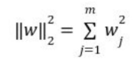
In L2 (Ridge) regularization, the regression coefficients are found by minimizing the L2 loss function and in L1 (Lasso) regularization, they're found by minimizing the L1 loss function which are given below.
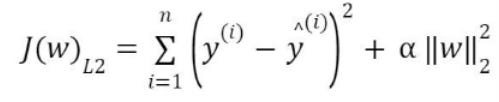
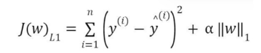
The L2 loss function is differentiable and hence, Ridge (L2) has an edge over Lasso (L1). There’s a mixing parameter beta in the elasticnet (EN) that balances L1 and L2 to get the best of both appraoches. When alpha is zero, we’re back to ridge and when alpha is 1, we’re back to lasso.
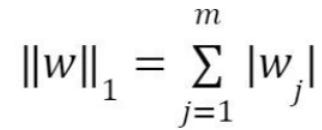
L2 regression retains all features, reducing the impact of less relevant features by shrinking their coefficients, L1 regression can set some coefficients to zero, effectively selecting a subset of most relevant features. If higher number of coefficients are forced to zero, it tends to increase the bias in the model. So tuning alpha ([0, 1]) to low values ensures the bias-variance tradeoff is well dealt with.
💡 Bias-variance tradeoff
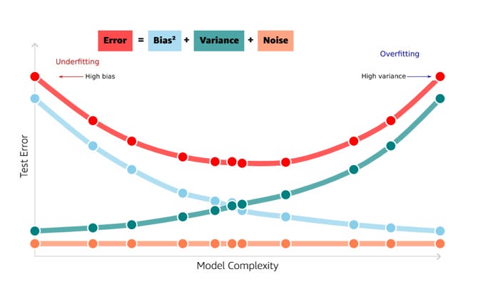
We see the relationship between bias and variance in prediction (test) error:
Error = Variance + Bias^2 + NoiseThe irreducible error term is the noise that cannot fundamentally be reduced by any model. The variance term is a function of the irreducible error, variance measures how much on an average, predictions vary for a given data point. The bias term is a function of how rough the model space is that is, how quickly in reality do values change as we move through the variable/feature space. The rougher the space, the faster the bias term increases. We can think of bias as measuring a systematic error in prediction.
In a world with imperfect models and finite data, there is a tradeoff between minimizing bias and variance.
💡 Low complexity & underfitting: Our model’s so simple, it fails to adequately capture the relationships in the data. The high test error is a direct result of the lack of complexity in the model.
💡High complexity & overfitting: Our model’s so specific to the data on which it was trained that it’s no longer applicable to different datasets. In other words, our model’s so complex that instead of learning true trend underlying the dataset, it memorizes noise, as a result of which the model is not generalizable to unseen dataset (beyond training data).
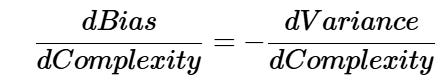
As an example, if more polynomial terms are added to a linear regression model, the resulting model complexity increases which in turn, means bias has a negative first-order derivative/slope in response to model complexity while variance has a positive slope. In effect, the sweet spot for any model is the level of complexity at which the increase in bias is equivalent to the reduction in variance.
If the model complexity exceeds this sweet spot, we are over-fitting while if the complexity falls short of the sweet spot, we are under-fitting. In practice, there is no analytical way to find this spot. Classic example of bias-variance tradeoff is the kNN algorithm.
We must explore differing levels of model complexity, and then choose the complexity (level) that minimizes the (test/prediction) error.
🎯 Model Assessment
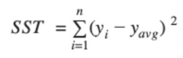
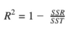
The sum of squared residuals (SSR) is a loss function, same as a model evaluation metric. The goodness of fit is R^2, represented in terms of SSR (or SSE) and SST (total sum of squares). R^2 increases if the degree of freedom (n-m-1) of the dataset decreases and hence, the model loses its reliability.
Please note that (n-1) is the degree of freedom for a single parameter or variable coefficient to be estimated. Degree of freedom is the number of independent parameters that a statistical analysis can estimate, in short the number of parameters free to vary.
Additional model complexity is penalized with adjusted R2 . Its value increases from R^2 when the new term improves the fit and decreases from R^2 when the term doesn’t improve the fit. In other words, adj. R^2 compensates/adjusts for inclusion of an irrelevant or unrelated variable term in the model and therefore, is an appropriate metric for model evaluation.
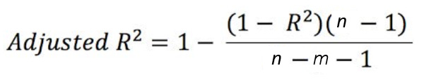
A variation in the independent (predictor x) variable explains a variation in the dependent (response y) variable. Adjusted R^2 is more accurate as it considers only significant predictors. Zero linear relationship between x and y yields adj. R^2 = 0 and adj. R^2 = 1 means 100% variation in y is explained by variation in x. A negative R^2 means that our model is doing worse (capturing less variance in y) than a flat line through the mean of our data would.

However, use of adjusted R^2 is less generalizable and may still overfit the data. Resampling methods (e.g. cross-validation) can be used to accurately measure prediction error.